Viral Transmission Model
import pandas as pd
import numpy as np
import pylab as plt
import datetime

import scipy.optimize as spo
import scipy.integrate as spi
Data Preprocessing
The dataset we will be using is the Global Coronavirus (COVID-19) Data (Corona Data Scraper) provided by Enigma.
AWS product link Corona Data Scraper page
We are only interested in the state-level data in United States. To save time from opening a super large dataset, we save each state's data into small files.
df = pd.read_csv("datasets/timeseries.csv")
df_US = df[(df["country"]=="United States") & (df["level"]=="state")]
df_US = df_US[["state", "population", "cases", "deaths", "recovered", "tested", "hospitalized", "date"]]
states = np.unique(df_US["state"])
for state in states:
    df_US[df_US["state"]==state].to_csv("datasets/timeseries_states/"+state+".csv", index=0)
State Data Snapshot
def chooseState(state, output=True):
    df_state = pd.read_csv("datasets/timeseries_states/"+state+".csv")

    ### data cleaning

    # some col is missing in some state's report
    na_cols = []
    for col in df_state.columns.values:
        if df_state[col].isna().all():
            na_cols.append(col)
    for col in na_cols:
        df_state = df_state.drop(col, axis=1)

    # some data is missing at the beginning of the outbreak
    suggest_startdate = df_state.iloc[0]["date"]
    for i in range(len(df_state.index)):
        if df_state.iloc[i].notna().all():
            suggest_startdate = df_state.iloc[i]["date"]
            break

    # regulate the data
    df_state = df_state.fillna(0)
    df_state["date"] = pd.to_datetime(df_state["date"])


    if output:
        ### snapshot and mark data inconsistency
        plt.figure()
        plt.title(state)
        for line, style in [ ("cases", "-b"), ("deaths", "-k"), ("recovered", "-g")]:
            if line in df_state.columns.values:
                plt.plot(df_state[line], style, label=line)
                for i in range(1, len(df_state.index)):
                    if abs(df_state[line][i] - df_state[line][i-1]) > (max(df_state[line]) - min(df_state[line])) / 6:
                        plt.plot(i, df_state[line][i], "xr")
        plt.legend()

        ### print out data-cleaning message
        if na_cols == []:
            print("Data complete, ready to analyze.")
        else:
            print("Data incomplete, cannot analyze.")
            print("NA cols: ", na_cols)
        print("Suggest choosing start date after", suggest_startdate)

    ### discard the outliers
    for line in [ "cases", "deaths", "recovered", "hospitalized"]:
        if line in df_state.columns.values:
            col_idx = list(df_state.columns).index(line)
            for i in range(1, len(df_state.index)-1):
                if (df_state.iloc[i, col_idx] - df_state.iloc[i-1, col_idx]) * (df_state.iloc[i+1, col_idx] - df_state.iloc[i, col_idx]) < -((max(df_state[line]) - min(df_state[line])) /4)**2:
                    df_state.iloc[i, col_idx] = (df_state.iloc[i-1, col_idx] + df_state.iloc[i+1, col_idx]) / 2
                    if output:
                        plt.plot(i, df_state[line][i], "or")

    return df_state, na_cols, suggest_startdate
For example, we are interested in New York state.
state = "New York"
df_state, _, _ = chooseState(state)
df_state.sample(5).sort_values("date")

For example, we are interested in the first two weeks in April.
def chooseTime(df_state, start_date, end_date):
    start = np.datetime64(start_date)
    end = np.datetime64(end_date)

    # The time period of interest
    sample = df_state[ (df_state["date"] >= start) & (df_state["date"] <= end) ]
    # The future period to determine "exposed"
    sample_future = df_state[ (df_state["date"] >= start + np.timedelta64(14,'D')) & (df_state["date"] <= end + np.timedelta64(14,'D')) ]

    return sample, sample_future
start_date, end_date = "2020-04-01", "2020-04-14"
sample, sample_future = chooseTime(df_state, start_date, end_date)
SEIR Infection Model
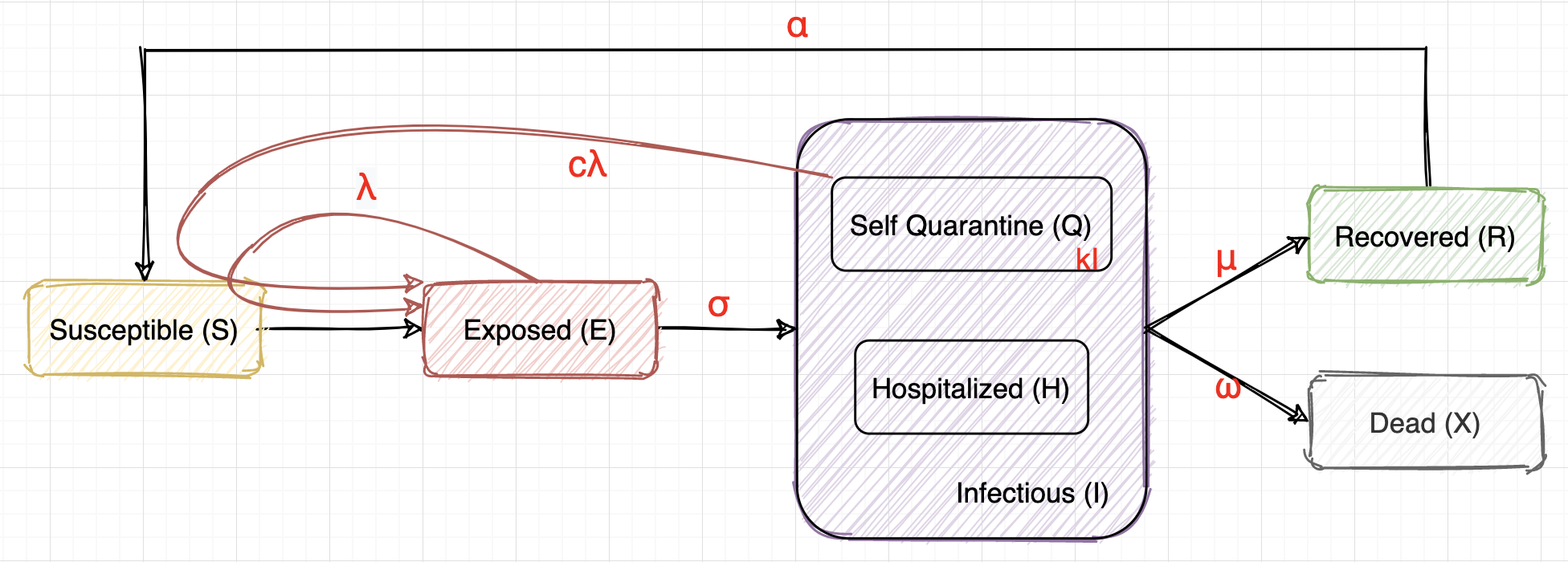
We can use an SEIR model to describe the transmission dynamics of Covid19 as above.
We Assume...
- Susceptible (S): healthy people, will be infected and turn into E after close contact with E or Q.
- Exposed (E): infected but have no symptoms yet, infectious with a rate of $\lambda$. E will turn into I after the virus incubation period, which is 14 days on average. So we assume $\sigma = 1/14$, dE/dt (t) = dI/dt (t+14).
- Infectious (I): infected and have symptoms. We will take the data of test_positive or cases_reported as the data of I. The severe cases will be hospitalized (H), the mild cases will be in self quarantine (Q). I may recover or die after some time.
- Self Quarantine (Q): have symptoms, may still have some contact with others, thus infectious with a different rate of $c\lambda$ ($0 \le c \le 1$). We also assume $Q = kI$, where $k = 1 - avg(\frac{\Delta hospitalized}{\Delta test\_pos}) $
- Hospitalized (H): have symptoms, kept in hospitals, assume no contact with S.
- Recovered (R): recovered and immune, may turn into S again (immunity lost or virus not cleared)
- Dead (X): dead unfortunately :(
Therefore, we have a set of differential equations to describe this process:
$\begin{aligned} &\frac{dS}{dt}& &=& - \lambda \frac{S}{N} E - c\lambda \frac{S}{N} Q + \alpha R ~~~ &=& - \lambda \frac{S}{N} E - c\lambda \frac{S}{N} kI + \alpha R \\ &\frac{dE}{dt}& &=& \lambda \frac{S}{N} E + c\lambda \frac{S}{N} Q - \sigma E ~~~ &=& \lambda \frac{S}{N} E + c\lambda \frac{S}{N} kI - \sigma E \\ &\frac{dI}{dt}& &=& \sigma E - \mu I - \omega I \\ &\frac{dX}{dt}& &=& \omega I \\ &\frac{dR}{dt}& &=& \mu I - \alpha R \end{aligned}$
$S + E + I + R + X = N,~ I = Q + H$
Apply to our datasets, we have:
$ R = recovered,~ X = deaths,~ I = test\_pos - deaths - recovered,\\ E(t) = I(t+14) - I(t),~ S = N - E - I - R - X,\\ k = 1 - avg(\frac{\Delta hospitalized}{\Delta test\_pos}) $
### run SEIR model on sample data

def SEIR(sample, sample_future, output=True):

    ### differential equations for spi.odeint, INP - initial point, t - time range
    # dS/dt = - lamda*S/N*E - c*lamda*S/N*k*I + alpha*R
    # dE/dt =   lamda*S/N*E + c*lamda*S/N*k*I - sigma*E
    # dI/dt = sigma*E - miu*I - omega*I
    # dX/dt = omega*I
    # dR/dt = miu*I - alpha*R
    def diff_eqs(INP, t, lamda_p, c_p, alpha_p, omega_p, miu_p):
        Y = np.zeros((5))
        V = INP
        Y[0] = - lamda_p*V[0]/N*V[1] - c_p*lamda_p*V[0]/N*k*V[2] + alpha_p*V[4]
        Y[1] =   lamda_p*V[0]/N*V[1] + c_p*lamda_p*V[0]/N*k*V[2] - sigma*V[1]
        Y[2] = sigma*V[1] - miu_p*V[2] - omega_p*V[2]
        Y[3] = omega_p*V[2]
        Y[4] = miu_p*V[2] - alpha_p*V[4]
        return Y

    ### cost function for optimization
    def MSE(params):
        INP = (S[0], E[0], I[0], X[0], R[0])
        t_range = np.arange(0, len(S), 1)
        RES = spi.odeint(diff_eqs, INP, t_range, args=tuple(params))
        mse = 0
        for i in range(len(S)):
            mse += ( (RES[i,0] - S[i]) ) **2
            mse += ( (RES[i,1] - E[i]) ) **2
            mse += ( (RES[i,2] - I[i]) ) **2
            mse += ( (RES[i,3] - X[i]) ) **2
            mse += ( (RES[i,4] - R[i]) ) **2
        mse = mse / len(S)
        return mse


    ### get necessary data from dataset

    cases = np.array(list(sample["cases"])) # test_positive
    cases_future = np.array(list(sample_future["cases"])) # to calculate exposed
    hospitalized = np.array(list(sample["hospitalized"])) # to calculate k
    deaths = np.array(list(sample["deaths"])) # X
    recovered = np.array(list(sample["recovered"])) # R
    N = np.mean(df_state["population"])

    X = deaths
    R = recovered
    I = cases - deaths - recovered
    E = cases_future - cases
    S = N - E - I - X - R

    dS = S[1:] - S[:-1]
    dE = E[1:] - E[:-1]
    dI = I[1:] - I[:-1]
    dX = X[1:] - X[:-1]
    dR = R[1:] - R[:-1]
    S = S[:-1]
    E = E[:-1]
    I = I[:-1]
    X = X[:-1]
    R = R[:-1]


    ### guess params
    # By experience: k, sigma
    k = 1 - np.mean( (hospitalized[1:]-hospitalized[0:-1] +1e-5) / (cases[1:]-cases[:-1] +1e-5) ) # k = deltaH / deltaCases
    sigma = 1/14 # virus incubation period = 14 days
    # From optimization: lamda, c, alpha, omega, miu
    alpha0 = 0.006
    omega0 = np.mean((dX+1e-5) / (I+1e-5)) # dx/dt = omega*i
    c0 = 0.4
    lamda0 = np.mean(- (dS - alpha0*R +1e-5) / (S/N * (E+c0*k*I) +1e-5) ) # dS/dt = - lamda*S/N*(E+ckI) + alpha*R
    miu0 = np.mean((dR + alpha0*R +1e-5) / (I+1e-5)) # dr/dt = miu*i - alpha*r

    ### Optimization to find best params
    params0 = (lamda0, c0, alpha0, omega0, miu0) # lamda, c, alpha, omega, miu
    ret = spo.minimize(MSE, params0, bounds=[(0,1), (0,1), (0,1), (0,1), (0,1)])
    params = ret.x
    params0 = [round(i,8) for i in params0]
    params = [round(i,8) for i in params]
    k = round(k,8)
    sigma = round(sigma,8)

    if output:
        print("Estimated k: ", k, "; sigma: ", sigma)
        print("Optimization for lamda, c, alpha, omega, miu")
        print("params0: ", params0)
        print("params: ", params)

        ### solve ode and plot
        INP = (S[0], E[0], I[0], X[0], R[0])
        t_range = np.arange(0, len(S)*5, 1)
        RES = spi.odeint(diff_eqs, INP, t_range, args=tuple(params))

        plt.figure(figsize=(10,6))

        plt.plot(RES[:,1], '-b', label='E_predict')
        plt.plot(RES[:,2], '-r', label='I_predict')
        plt.plot(RES[:,3], '-k', label='X_predict')
        plt.plot(RES[:,4], '-g', label='R_predict' )
        plt.plot(E, "xb", label="E_real")
        plt.plot(I, "xr", label="I_real")
        plt.plot(X, "xk", label="X_real")
        plt.plot(R, "xg", label="R_real")

        plt.grid()
        plt.xlabel('Time', fontsize = 12)
        plt.ylabel('number of people', fontsize = 12)
        plt.legend(loc=0)
        plt.title(state + ": " + str(start_date) + " - " + str(end_date), fontsize = 14)
        plt.show();

    return params, k, sigma
params = SEIR(sample, sample_future)

Example1: California
state = "California"
df_state, _, _ = chooseState(state)
# df_state.sample(5).sort_values("date")

Everything seems fine (except that jump), then we choose an appropriate time period to analyze
start_date, end_date = "2020-05-15", "2020-05-28"
sample, sample_future = chooseTime(df_state, start_date, end_date)
params = SEIR(sample, sample_future)

Example2: New York
state = "New York"
df_state, _, _ = chooseState(state)
# df_state.sample(5).sort_values("date")
Everything seems fine, then we choose an appropriate time period to analyze.
start_date, end_date = "2020-05-01", "2020-05-14"
sample, sample_future = chooseTime(df_state, start_date, end_date)
params = SEIR(sample, sample_future)

Example3: Illinois
state = "Illinois"
df_state, _, _ = chooseState(state)
# df_state.sample(5).sort_values("date")

There are too many missing data (no recovered) for Illinois, we can not analyze now.
Example4: Texas
state = "Texas"
df_state, _, _ = chooseState(state)
# df_state.sample(5).sort_values("date")

The hospitalized data is missing, we may use the average k instead. But we can not analyze now.
Generate state-time-params data
Now that our SEIR infection model is working, we choose some states of interest and compute the corresponding optimal parameters for further modeling.
StateOfInterest = ["Arizona", "California", "Minnesota", "New Mexico", "New York",
                   "Oklahoma", "South Carolina", "Tennessee", "Utah", "Virginia",
                   "West Virginia", "Wisconsin"]

df_SOI = pd.DataFrame(columns = ["state", "startdate", "enddate", "k", "sigma", "lamda", "c", "alpha", "omega", "miu"])

for state in StateOfInterest:
    df_state, _, suggest_startdate = chooseState(state, False)

    # choose 15 days as a period
    if np.datetime64(suggest_startdate,'D') - np.datetime64(suggest_startdate,'M') <= np.timedelta64(14,'D'):
        real_startdate = np.datetime64(suggest_startdate,'M') + np.timedelta64(15,'D')
    else:
        real_startdate = np.datetime64(np.datetime64(suggest_startdate,'M') + np.timedelta64(1,'M'), 'D')

    stopdate = np.datetime64("2020-07-01")
    startdate = real_startdate

    while True:
        if startdate > stopdate:
            break
        enddate = startdate + np.timedelta64(14,'D')

        sample, sample_future = chooseTime(df_state, startdate, enddate)
        params = SEIR(sample, sample_future, False)

        df_SOI = df_SOI.append([{"state":state, "startdate":startdate, "enddate":enddate, "k":params[1], "sigma":params[2], "lamda":params[0][0], "c":params[0][1], "alpha":params[0][2], "omega":params[0][3], "miu":params[0][4]}], ignore_index=True)

        if np.datetime64(startdate,'D') - np.datetime64(startdate,'M') <= np.timedelta64(0,'D'):
            startdate = np.datetime64(startdate,'M') + np.timedelta64(15,'D')
        else:
            startdate = np.datetime64(np.datetime64(startdate,'M') + np.timedelta64(1,'M'), 'D')
df_SOI.to_csv("datasets/model_out.csv", index=0)
df_SOI.sample(5)